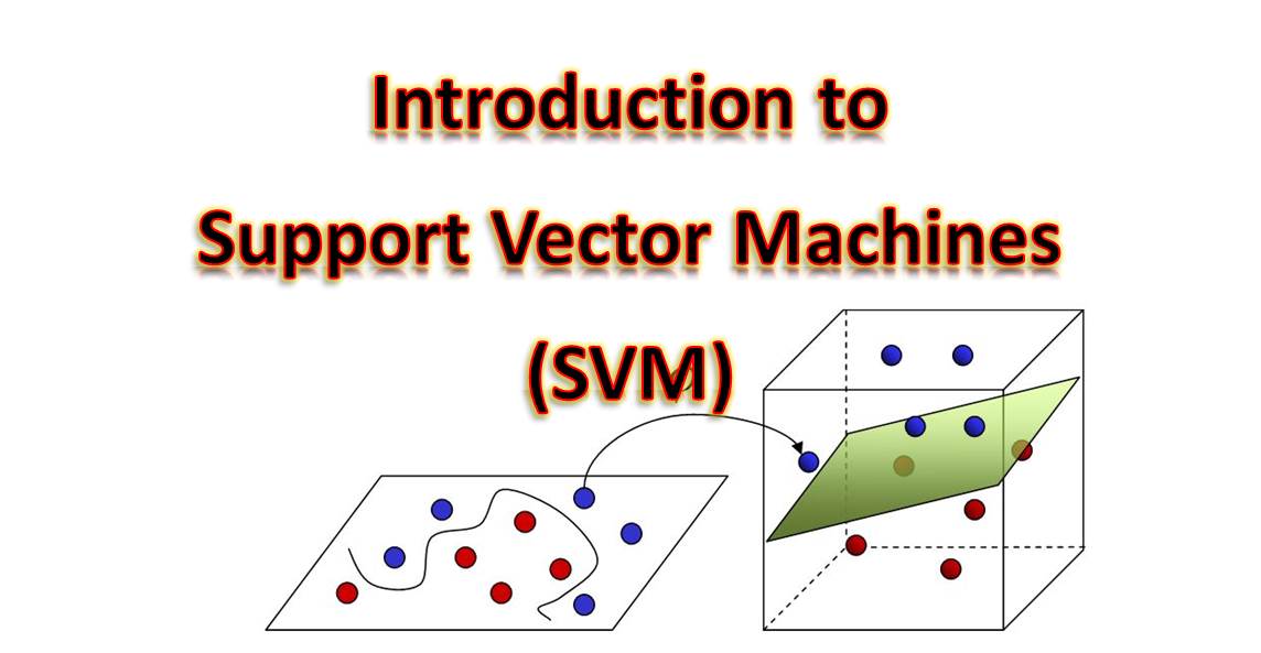
Support Vector Machines (SVM) are powerful machine learning algorithms used for classification and regression tasks. SVMs are based on the concept of finding an optimal hyperplane that separates data points belonging to different classes with the largest possible margin. SVM has gained significant importance in the field of machine learning due to its effectiveness in handling complex datasets and its ability to generalize well to unseen data. It has found applications in various domains such as image classification, text analysis, bioinformatics, and finance.

SVM’s versatility and robustness make it a popular choice for many real-world problems. This article provides a comprehensive overview of Support Vector Machines (SVM). It covers the fundamental concepts of SVM, both linear and non-linear approaches, the training process, evaluation and decision-making, handling imbalanced data, advantages, and limitations of SVM, extensions and variants, and practical applications of SVM.
Basic Concepts of SVM
A. Binary Classification Problem
SVM primarily deals with binary classification problems, where the objective is to classify data points into one of two classes. The decision boundary or hyperplane separates the data points belonging to different classes. The Full Stack Developer Course is great for learning more fundamentals.
B. Hyperplane and Decision Boundary
The hyperplane in SVM is a decision boundary that separates the data points. In two-dimensional space, the hyperplane is a line; in higher-dimensional spaces, it becomes a hyperplane. SVM aims to find the hyperplane that maximizes the margin, the distance between the hyperplane and the closest data points from each class.
C. Maximum Margin Principle
The maximum margin principle in SVM states that the best decision boundary is the one that maximizes the margin between the classes. SVM finds the optimal hyperplane by maximizing the distance between the support vectors, which are the data points closest to the decision boundary.
D. Linearly Separable and Non-linearly Separable Data
SVM can handle both linearly separable and non-linearly separable data. In the case of linearly separable data, a linear hyperplane can perfectly separate the classes. However, when the data is not linearly separable, SVM employs the kernel trick to map the data into a higher-dimensional feature space where it becomes linearly separable.
Linear SVM
A. Linearly Separable Data
Linear SVM works well when a linear hyperplane can separate the data points belonging to different classes. It aims to find the hyperplane that maximizes the margin between the classes.
B. Formulation of SVM Optimization Problem
The optimization problem in linear SVM involves finding the coefficients of the hyperplane that minimize the classification error and maximize the margin. This is done by solving a quadratic programming problem.
C. Soft Margin SVM for Handling Misclassified Points
Soft margin SVM allows for some misclassified data points. It introduces slack variables that allow data points to be on the wrong side of the margin or even on the wrong side of the hyperplane. The C-parameter controls the trade-off between margin maximization and minimizing misclassifications.
D. Slack Variables and C-parameter
Slack variables in soft margin SVM represent the degree of misclassification. The C-parameter determines the balance between maximizing the margin and minimizing the misclassification error. A higher value of C leads to a stricter classification, while a lower value allows more misclassifications.
Non-linear SVM
A. Kernel Functions
Kernel functions are used in non-linear SVM to transform the data into a higher-dimensional feature space where it becomes linearly separable. Various kernel functions, such as the Radial Basis Function (RBF) kernel, polynomial kernel, or sigmoid kernel, can be employed to capture complex relationships between data points.
B. Radial Basis Function (RBF) Kernel
The RBF kernel is commonly used in non-linear SVM. It measures the similarity between data points based on their Euclidean distance. The RBF kernel allows SVM to handle complex, non-linear decision boundaries.
C. Polynomial Kernel
The polynomial kernel maps the data into a higher-dimensional space using polynomial functions. It captures non-linear relationships between data points by computing polynomial terms of the features.
D. Other Kernel Functions
In addition to RBF and polynomial kernels, SVM supports various other kernel functions, such as the sigmoid kernel, linear kernel, and custom kernels. The choice of the kernel function depends on the nature of the data and the complexity of the decision boundary.
Conclusion
Support Vector Machines (SVM) are powerful machine learning algorithms that have made a significant impact in various domains. SVMs excel in both binary classification and regression tasks, providing robust and accurate predictions. By finding an optimal hyperplane or decision boundary, SVM maximizes the margin between data points of different classes, resulting in good generalization and effective separation.
